After completing this lesson, you’ll be able to:
As mentioned in Learn Spatial Data Concepts, spatial analysis tries to describe, explore, and explain patterns and relationships of topology, geography, and geometry. We use spatial analysis techniques to answer questions about relationships between objects by filtering, measuring, and overlaying spatial data.
We've already looked at filtering and overlaying, but other spatial analysis techniques can be helpful. The methods covered in this lesson let you modify the structure of your spatial data.
FME includes over 40 spatial analysis transformers. Here, we will introduce a few of the most popular ones.
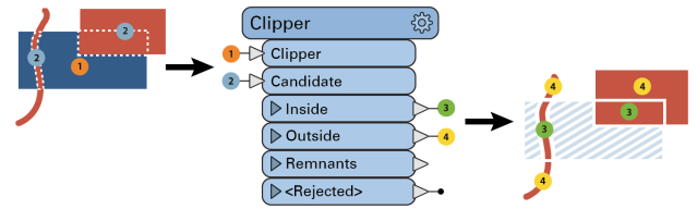
The Clipper takes two sets of spatial data as inputs. You can think of it as a cookie-cutter. One (the Clipper) is the cutter. The other (the Candidate) is the cookie. The clipper stamps out shapes in the candidate, creating a new dataset that is the candidate cut to the clipper's boundaries.
This diagram illustrates area-on-line and area-on-area vector clipping results.
Both the line and area Candidates are split where they cross the Clipper boundary, and the results are output:
In terms of set theory, the Clipper looks at the intersection of two data streams.
The Clipper helps you change the boundaries of your data. For example, say you had a dataset of point locations of all the fire halls in a state. If you wanted to extract just the fire halls within a particular city, you could use a polygon of the city boundaries as the clipper and the fire halls as the candidates.
You can also use the Clipper in combination with other spatial analysis transformers. For example, from the example above, say you wanted to know how many schools were within 500 meters of the fire stations. You could use a Bufferer (see below) to create polygons representing all the areas within 500 meters of the fire stations. Then, you could use the Clipper with the buffered area as the Clipper and the schools as the Candidate.
As is usually the case with FME, there are many ways to conduct spatial analysis. You could accomplish the same procedure using the NeighborFinder, with the schools as the Base and the fire stations as the Candidate. Either way is valid.
The Bufferer creates a buffer zone of specified size around or inside input geometry.
Its uses include:
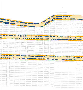
In this example, we buffered arterial roads (shown in blue) to find address points (shown in green) within a fixed distance. Then, we connected the buffered roads and address points to a SpatialFilter, identifying the addresses within the buffers (blue points).

The Dissolver removes common boundaries to create larger areas. This transformer accepts two-dimensional polygonal features, including donuts, and can optionally accumulate input attributes.
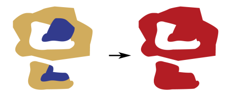
The Dissolver forms dissolved polygons along shared edges, removing interior boundaries between adjacent polygons. A common use case for this transformer is simplifying many small features into a larger single feature. For example, combining multiple counties creates a single polygon representing the state.
In terms of set theory, the Dissolver creates a union of multiple streams of features.
The example below shows areas before and after we used a Dissolver transformer on our data.
The Aggregator combines feature geometries into heterogeneous or homogeneous aggregates. Alternatively, it combines feature attributes without any geometry.
The example below illustrates a geometric feature of diverse attributes on the left and its aggregated output on the right.

The Aggregator is commonly used to combine features into an aggregate when building a hierarchical geometry model. For example, you might have a 3D CAD drawing of a house, with the House itself being an aggregate. It contains more aggregates, including Roof and Walls. The Walls are also an aggregate containing four faces. You can use the Aggregator to build these aggregate geometries.
You might use the Aggregator if you have a dataset with duplicate polygons of a state's counties but want to combine them so you have only a single polygon per county. There are options to control how attributes are combined. The Aggregator is often used with a Group By parameter to control how the transformer aggregates features. In the county example, the Group By would be an attribute storing the county's name or ID.
You can use the Aggregator on features with or without geometry.
